Advances in Model Based Reinforcement Learning
Reinforcement learning is a very interesting research topic, in recent years, their applications and their performance have been growing quickly. In this blog post, we present the basics of model-based reinforcement learning and its recent advances.
Introduction
Model-based reinforcement learning is a branch in Reinforcement Learning where the transition function $$P(s’, r|s, a)$$ in the Markov decision process (MDP) is used. This model is used to improve or create a policy (planning), where the value function is calculated as an intermediate step, as can be seen in Figure 1 in the model-learning branch. Direct RL, means model-free RL where the policy or value-function is computed directly from experience and it is not needed to model the dynamics. However, these kinds of methods are too poor sample efficient due to that these methods rely on the probability to find good interactions, this becomes even more complicated when the environment has high dimensional state-action space and when sparse rewards are presented. In contrast, recent advances in Model-based RL, have shown capabilities to learn optimal policies with considerably fewer interactions, becoming methods more applicable to problems where exploration interactions are critical.
![Figure 1, Taken from [1]](https://ericktornero.github.io/blog/images/squeme_mbmf.png)
Figure 1, Taken from [1]
An interesting algorithm for starting the analysis of model-based reinforcement learning is called Dynamic Programming algorithm, where it is assumed a prior and exact knowledge of the dynamics (transition function). However, in the real world, the dynamics are usually unknown and can be very complex to model. For these kinds of problems, model learning with function approximators is used just as supervised learning with the collected transitions $$(s, a, s’)$$ as a dataset. Examples of these environments are shown Fig. 2, the left picture shows a Simple Gridworld example with a discrete state and actions. In this case the transition function is known, for example $$P(s_2|s_1,right)=1.0$$ and $$P(s_2|s_1, left)=0.0$$, where $$s_x$$: represents the slot $$x \in {0, 15}$$. In the right picture, an environment more approximate to the real world is shown: Halfcheetah in Mujoco Environment, where the dynamics of this environment is unknown and complex.
![Figure 2, left: Gridworld environment, taken from [1]. Right: Halfcheetah Environment](https://ericktornero.github.io/blog/images/gridworld_hchetaah.png)
Figure 2, left: Gridworld environment, taken from [1]. Right: Halfcheetah Environment
For low dimensional state-action space, Gaussian Process (GPs) can be used to approximate the transition function. However when complexity in the model increases, e.g. in robotics control, the gaussian process used to be inadequate. Neural Networks, however, is known for its high adaptability to complex functions, and in recent years, has been showed interesting results in several applications, such as image classification. In that sense, this post focus on the recent advances in MBRL that use Neural Networks for the approximation of the transition function.
Basic concepts in Model-Based Reinforcement Learning
Reinforcement learning Framework is defined over a Markov Decision Process, and elements in an MDP are defined in the tuple $$(\mathcal{S}, \mathcal{A}, \mathcal{R}, p, \gamma)$$, where $$\mathcal{S}$$ is the state space, $$\mathcal{A}$$ is the action space, $$\mathcal{R}$$ is the reward and $$p(s’, r|s, a)$$ define the transition function. In Fig. 3, the interaction interaction agent-envrionment is shown, given an observed state $$s_t \in \mathcal{S}$$ at any particular timestep $$t$$, the agent take an action $$a_t \in \mathcal{A}$$ drawn from its policy $$\pi(a_t|s_t)$$. The environment respond with the next state $$s_{t+1}$$ and the reward $$r_{t+1}$$ produced by take action $$a_t$$.

Figure 3, Interaction in MDP
Either model-based or model-free methods aim to compute a policy $$\pi(a|s)$$ that maximizes the expected reward. In the case of mode-based, the policy is computed indirectly by using the transition model $$p(s’,r|s, a)$$ for planning. Dynamic Programming are considered as model-based methods since it uses its prior knowledge of the dynamics. This is used to improve the value-function, in Equation (a) is shown the update rule for the value function for the Policy Iteration algorithm.
$$v(s) \xleftarrow{} \sum_{s’, r} p(s’, r|s,\pi(s))[r + \gamma v(s’)] \tag{a}$$
However, in Dynamic Programming is assumed an exact knowledge of the dynamics. In the real world, the dynamics are usually unknown. To overcome this problem, methods tend to ignore the transition function $$p(s’, r|s, a)$$, instead try to compute the expected value function through experience, e.g. Q-Learning. On the other hand, instead of having a backup of the value function, one can use the transition function and used to compute candidates of trajectories, these algorithms are known as shooting algorithms. In this blog, we take care of the second type of method. In that sense, the following part of this blog shows recent advances in this field. We will explain more about shooting methods in another post.
Neural network dynamics for model-based deep reinforcement learning with model-free fine-tuning
Anusha Nagabandi et al. UC Berkeley 2017
This paper proposes deterministic Neural Network for Model-based Reinforcement Learning for solving continuous taks. The pipeline is shown in Fig. 4, a Neural Network $$\hat{f}\theta$$ models the dynamics of the environment and is trained as a multidimensional regression in a deterministic way using MSE Loss function (Eq. 3). The MPC Controller laverage the knowledge of the transition function $$\hat{f}{\theta}$$ to predict the next state $$\hat{s}{t+1}$$ given a current state $$s_t$$ and an action taken $$a_t$$ as in Eq. 1. The same logic is used for multistep prediction of horizon $$H$$, by recursively applying the Eq. 1 $$H$$ times (Eq. 2). Note that reward is a function over states $$r_t = fn(s_t)$$, then if the state $$\hat{s}{t+i}$$ is predicted by Eq. 2, reward is approximate by $$\hat{r}{t+i} = fn(\hat{s}{t+i})$$.
$$\hat{s}{t+1} = s_t + \hat{f}\theta(s_t, a_t)\tag{1}$$
$$\hat{s}{t+i} = \hat{f}\theta(\dots(\hat{f}\theta(\hat{f}\theta(s_t, a_t), a_{t+1})\dots, a_{t+i-1}) \tag{2}$$
$$Loss_\theta = \frac{1}{\mathcal{D}} \sum_{(s_t, a_t, s_{t+1}) \in \mathcal{D}} \frac{1}{2} \Vert (s_{t+1} - s_t) - \hat{f}_\theta(s_t, a_t) \Vert^2 \tag{3}$$
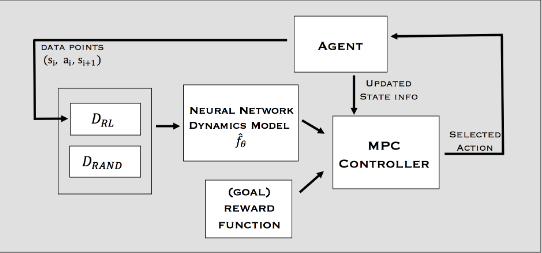
Figure 4, Pipeline Anusha paper. MPC Controller is a trajectory optimizer for planning future H actions, given a known transition function p(s’|s, a) and a reward function r_t = fn(s_t). The MPC just take the first action of the trajectory and replan for each time-step. Transition tuple (s_i, a_i, s_{i+1}) is stored in a dataset D for train the Dynamics with supervised learning and MSE Loss.
This method reaches acceptable results in continuous tasks, It was tested in the Mujoco Environment. While this method takes over 100x fewer samples concerning model-free methods, this method can not reach the same asymptotic performance. A second proposal uses the previous model-based for initializing a model-free method (PPO), this is particularly useful for model-free because the sample-complexity of model-free based on the probability to see good interactions, and model-based can achieve this with few samples. The results show faster convergence for model-free methods as can be seen in Fig. 5 and Fig. 6 (fine-tuning).
Figure 5, Performance of Model-based method (left) vs Model-free with fine-tuning (right), acceptable performance is shown for model-based with just thousands of samples, model-free shown high performance in the convergence (millions of samples).
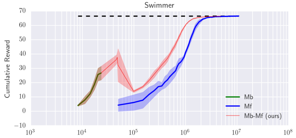
Figure 6, Performance Model-free with fine-tuning (red) vs Model-free (blue) in the Swimmer environment. Here, greater sample efficiency of applying fine-tuning over the previous model-based is shown. We can appreciate that is difficult or impossible for a simple model-free method to achieve the performance of a Model-based method with the same number of samples, this feature is taken in advantage to make fine-tuning
Deep Reinforcement Learning with a handful of trials with probabilistic models
Kurtland Chua et al. UC Berkeley 2018
This paper achieves interesting results reducing the gap between model-free and model-based RL in asymptotic performance with 10x fewer sample iterations required, by mixing some ideas to model the uncertainty of the dynamics: These uncertainties are divided into two:
1. Aleatoric Uncertainty:
This uncertainty is given by the stochasticity of the system, e.g. noise, inherent randomness. The paper models this behavior by outputting the mean and variance of a Gaussian Distribution, It allows us to model different variances for different states (Heterokedastic). While the distribution over states can be assumed any tractable distribution, this paper assumed a Gaussian Distribution over states. Given by:
$$\hat{f} = Pr(s_{t+1}|s_t, a_t) = \mathcal{N}(\mu_\theta(s_t, a_t), \Sigma{_\theta}(s_t,a_t))$$
In that sense the loss function is given by:
$$loss_{Gauss}(\theta) = \sum_{n=1}^N[\mu_\theta(s_n, a_n) - s_{n+1}]^\intercal \Sigma_\theta^{-1}(s_n, a_n)[\mu_\theta(s_n, a_n) - s_{n+1}] + \dots \ \dots + \log\det\Sigma{_\theta}(s_n, a_n)$$
2. Epistemic Uncertainty:
This uncertainty is given by the limitation of data. Overconfidence in zones where there are not sufficient data-training points can be fatal for prediction, epistemic uncertainty tries to model this. The paper model this by using a simple bootstrap of ensembles. In Fig. 4, an example of two ensembles is shown (red and blue). In zones where there are data for training, the two ensembles behave very similarly, but in zones where not, for example between the two markable zones of data points, each ensemble can take different behavior, these differences represent the uncertainty due to the missing of data or epistemic uncertainty.
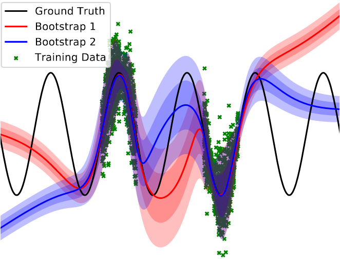
Figure 7, probabilistic Ensembles. Epistemic uncertainty can be seen in the center of the picture, where not data-training points appear, as a result, different behavior of the bootstrap ensembles exists. Aleatoric uncertainties can be seen in zones where there are many data-training points (Green) but still exits variance, proper of the environment.
Uncertainty propagation:
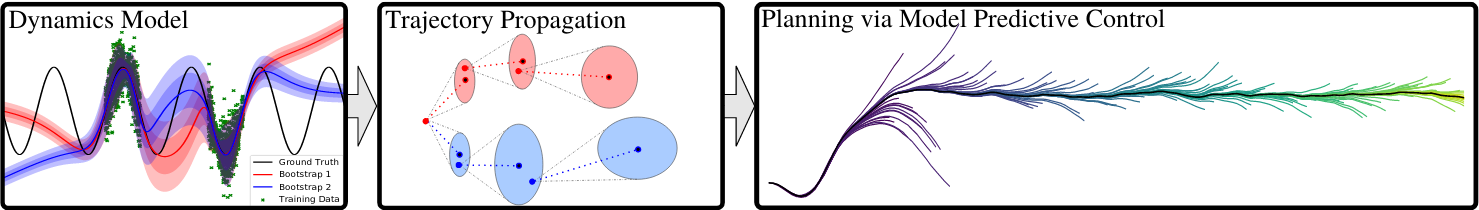
Figure 8, Pipeline. The algorithm uses both uncertainties previously presented for model the dynamics (left picture). These uncertainties are propagated through each sequence of trajectories by a particle system (center picture). The final reward for each timestep would the average of each particle at a given index. MPC controller, in this case, Cross-Entropy Method (CEM), propagate N candidates of sequences of horizon H and evaluate the best one trajectory, then, the first action of best trajectory is taken.
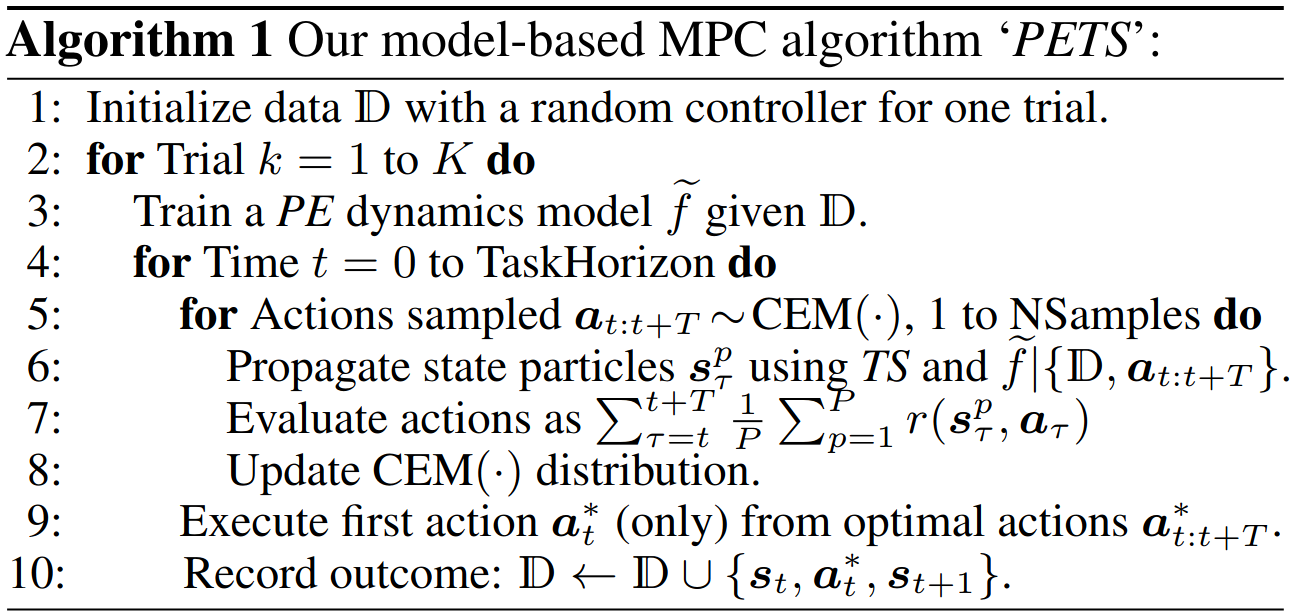
Figure 9, Algorithm: PETS
Deep Dynamics Models for Learning Dexterous Manipulation
Anusha Nagabandi et al. UC Berkeley 2019
This paper is an extension of the previous paper DRL with a handful of trials using probabilistic models (PETS), taking the problem of dexterous manipulation. It also models aleatoric and epistemic uncertainties with Gaussian parametrization via Neural Networks and with Ensembles bootstrap respectively. The main contributions are a modification for (MPPI) algorithm that uses weighted rewards. MPPI uses random sampling techniques to explore actions near to the control sequence, instead of in this paper a Filtering technique is used to add dependencies of previous timesteps:
Filtering and reward weighted refinement overview:
Given a sequence control:
$$(\mu_0, \mu_1, \dots, \mu_{H-1})$$
It is assumed that the control sequence is a future sequence of lenght $$H$$. This sequence is optimized every timestep and $$\mu_0$$ should be the control input to be taken at current timestep. Noises is added in the following way:
$$u_t^i \sim \mathcal{N}(0, \Sigma) \hspace{0.25cm} \forall i \in {0\dots N-1}, t \in {0\dots H-1}$$
$$n_t^i = \beta u_t^i + (1 - \beta) n_{t-1}^i \hspace{0.25cm}\text{where}\hspace{0.25cm} n_{t<0} = 0$$
Where $$u_t^i$$ is a gaussian noise with mean $$0$$ and $$\Sigma$$ covariance matrix and $$n_t^i$$ add dependence noise from the previous timestep.
Then each action for H (index $$t$$) horizon for N (index $$i$$) candidates is computed as:
$$a_t^i = \mu_t + n_t^i$$
With the previous actions sequence for N candidates, the predicted states are computed with the dynamics model, then the reward $$R_k$$ is computed for each trajectory. Then the new mean is computed through the weighted reward.
$$\mu_t = \frac{\sum_{k=0}^N (e^{\gamma R_k})(a_t^{(k)})}{\sum_{j=0}^N e^{\gamma R_j}} \hspace{0.25cm} \forall t \in {0\dots H-1}$$
Now, the new trajectory is optimized at $$\mu_{0: H-1}$$. Just the first action is taken: $$\mu_0$$ (Send to actuators).
Finally, the control sequence is updated, and the process is repeated for each timestep:
$$\mu_i = \mu_{i+1} \hspace{0.25cm} \forall i \in {0\dots H-2}, \hspace{0.25cm} \mu_{H-1} = \mu_{init}$$
Exploring Model-based Planning with Policy Networks
Tingwu Wang & Jimmy Ba, University of Toronto, Vector Institute 2019
This work is a derivation from the previous method presented (PETS). However, in this paper, it is used as a policy network to help in the planning task with iterative Cross-Entropy Method. Its main contribution is the proposal of an algorithm that has a better exploration of action-sequence candidates in the planning step.
Recall: In Gradient-free trajectory optimization (Random Shooting, CEM, MPPI, PDDM), it takes advantage of the knowledge of the dynamics $$p(s’|s, a)$$ by proposing several candidates (N) of action-sequences of length H. The way how these candidates are proposed (exploration) is the main concern of this paper.
In the following subsections, it is discussed how the algorithm search for trajectories: POPLIN-A (adding noise to actions) POPLIN-P (adding noise to parameters e.g. weights of a neural network). In both cases, the same heuristic of Iterative Cross-Entropy Method (CEM) are used (iteratively adjustment of gaussian distribution parameters to a group of elites which obtain the best rewards), but with the difference that POPLIN, uses a policy network to initialize action distribution instead of random actions as PETS.
Policy Planning in Action Space (POPLIN-A):
This algorithm uses Iterative Cross Entropy Method as PETS, however, istead of random initialization, it laverages the policy network to initializate distribution of action sequences. This initializations can be done in two ways:
POPLIN-A-Init: Be a$$i = {\hat{a}i, \hat{a}{i+1}\dots \hat{a}{i+H} }$$, a sequence of actions obtained by the iteration of the policy $$\hat{a}_t = \pi(\hat{s}t)$$ over the model $$ p(\hat{s}{t+1}| \hat{s}_t, \hat{a}_t)$$ starting from $$s_i$$. For the exploration process, Gaussian noise is added to this initial sequence, starting with $$\mu_0 = 0$$ and covariance $$\Sigma_0 = \sigma_0^2\mathcal{I}$$. Then this mean and covariance is iteratively updated by selecting $$\xi$$ elites, and computing the new mean and new covariance.
POPLIN-A-Replan: In POPLIN-A-Init, first, the action sequence is initialized, then the noise is added to this sequence. However in POPLIN-A-Replan, the first action is approximate by the policy, then noise is added to this action, the next state is computed taking into account this noise $$\hat{s}_{i+1} = p(\cdot | s_i, \pi(s_i) + \delta_i)$$.
Policy Planning in Parameter Space (POPLIN-P):
In planning in parameter space, Gaussian noise is added to the weights of the neural network. Then exploration is made in the following way:
$$\hat{a}i = \pi{\theta + \omega_t}(s_t)$$
$$\hat{s}_{t+1} = p(\cdot | s_t, \hat{a}_t)$$
Where $$\omega_t$$ is Gaussian noise, as in POPLIN-A, Gaussian noise parameters are updated with the Iterative CEM.
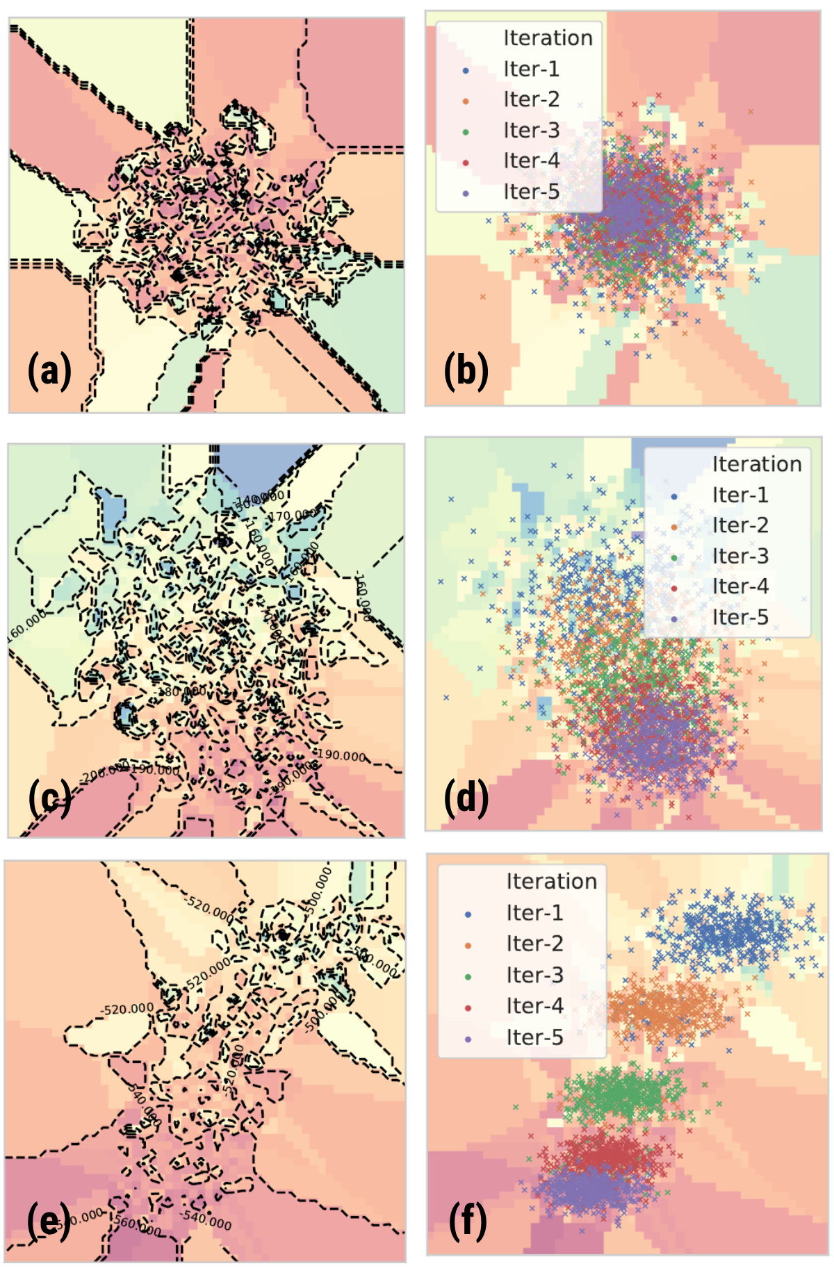
Figure 10, POPLIN surface comparison, Images in left side are the reward surface with respect (a) PETS, (c) POPLIN-A and (e) POPLIN-P. The Images in right side represent the action-sequence reduced with PCA projected in the reward surface relative to each left image
This paper found interesting results. In Fig. 10, If it is compared to the reward surface of the three algorithms (red color represents high reward). One can observe that the reward surface for the PETS algorithm has a lot of holes, it means that small portions of high reward appears rounded with portions of low reward. In consequence, the mean of action candidates over CEM iterations does not change significantly, it means a poor exploration of action sequences. However, for POPLIN algorithms, especially for POPLIN-P, the reward surface is smoother, allowing to the CEM algorithm a better exploration over iterations.
References
[1] R. Sutton, A. Barto. Reinforcement Learning: An Introduction, Second edition, 2018.
[2] A. Nagabandi et al. Neural Network Dynamics for Model-Based Deep Reinforcement Learning with Model-Free Fine Tuning. In ICRA 2018.
[3] K. Chua et al. Deep Reinforcement Learning in a Handful of Trials using Probabilistic Dynamics Models. In NIPS 2018.
[4] A. Nagabandi et al. Deep Dynamics Models for Learning Dexterous Manipulation. In CoRL 2019.
[5] Tingwu Wang et al. Exploring Model-based Planning with Policy Networks. Arxiv 2019.
Author Erick Tornero
LastMod 2020-01-30